Sequential Monte Carlo and the bootstrap filter

In the previous post I have outlined three possibilities for approximating the likelihood function of a state space model (SSM). That post is a required read to follow the topics treated here. I concluded with sequential importance sampling (SIS), which provides a convenient online strategy. However, in some cases SIS suffers from some numerical problems that I will address here. The key concept is the introduction of a resampling step. Then I introduce the simplest example of a sequential Monte Carlo (SMC) algorithm, the bootstrap filter. Recommendations on how to make best use of resampling are discussed.

Sequential Importance Sampling with Resampling

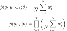
An important result derived in the previous post is the sequential update of the importance weights. That is, by denoting with $w_t^i$ the importance weight for particle $x_t^i$ we have

$w_t^i\propto \frac{p(y_t|x_t^i)p(x_t^i|x_{t-1}^i)}{h(x_{t}^i|x_{0:t-1}^i,y_{1:t})} w_{t-1}^i \qquad i=1,...,N.$

The weights update allows for an online approximation of the likelihood function of parameters $\theta$ , that we can write as

$\begin{aligned} \hat{p}(y_t|y_{1:t-1};\theta)&=\frac{1}{N}\sum_{i=1}^N w_t^i\\ \hat{p}(y_{1:T}|\theta)&= \prod_{t=1}^T\biggl (\frac{1}{N}\sum_{i=1}^N w_t^i\biggr ). \end{aligned}$

At this point, an approximate maximum likelihood estimate can be obtained by searching for the following (typically using a numerical optimizer)

$\hat{\theta} = \arg\max_\theta \hat{p}(y_{1:T}|\theta)$

or $\hat{p}(y_{1:T}|\theta)$ could be plugged into a Bayesian procedure for sampling from the posterior distribution $\pi(\theta|y_{1:T})$ (more on this in future posts).

Actually, while the procedure above can be successful, in general depending on the type of data and the adequacy of the model we employ to “fit” the data, some crucial problems can occur.

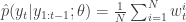
Particle degeneracy: the convenient representation of $w_t^i$ as a function of $w_{t-1}^i$ is problematic when particle $x_{t-1}^i$ produces a very small weight $w_{t-1}^i$ . With “very small” I mean that its numeric value as returned by a computer (floating point representation) is zero, even though its mathematical value is actually positive. This is because computers have a limited ability to represent very small and very large values: if a value is “too small” it will be represented as exactly zero on a computer, and if it is “too large” it will be represented as infinity. The former case, when $w_t^i$ is too small, is said to produce an underflow while a too large weight might produce an overflow. We focus on the underflow, as it is more common. Consider for example the plot below, where at time 44 there is a clear outlier, that is an observation with an unusual value compared to the rest of the data.

tsplot_weight_with_outlier_single_y_simple_4col-xml_graph_cmd1o1

This outlier could have been produced by an unusual statistical fluctuation, and at time $t=44$ the datum $y_{t}$ might be a realization from a tail of the distribution with density $p(y_{t}|x_{t})$ . While this is legitimate, numerically it can create issues for the stability of our calculations. Say that $p(y_{t}|x_{t})=N(y_t;x_t,0.5^2)$ , that is a Gaussian distribution with mean $x_t$ and standard deviation 0.5. Let’s see what happens if I anticipate some topic treated later on.

Say that I choose as importance density the transition density of the latent process, that is I set $h(x_{t}^i|x_{0:t-1}^i,y_{1:t}) \equiv p(x_{t}^i|x_{t-1}^i)$ , then the weight becomes

$w_t^i\propto N(y_t;x_t^i,0.5^2)w_{t-1}^i \qquad i=1,...,N$

with some abuse of notation. Now, for the given choice of proposal density (and if I have been employing a model appropriate for the data) then at the previous time instant 43, most particles will have values somewhere around 30 (see the y-axis in the figure), and we could expect that if $x_{43}^i\approx 30$ then most of the particles $x_{44}^i$ generated from $p(x_{44}^i|x_{43}^i)$ should take values not too far from 30. And here is a problem: from the figure we have $y_{44}\approx 4$ and the computer implementation for the density function of $N(y_{44};x_{44}^i,0.5^2)$ might underflow and return zero for many particles (I will describe some tricks mitigating this problem in a future post). Clearly, all those particles having zero weight doom the values of the descendant particles, because each weight depends on the previous one. A similar scenario could happen even without outliers, if we simulate from a model not appropriate for the data. Clearly, as the time horizon $T$ increases, it is not unlikely to incur in such a problem.

The phenomenon were most particles have very small weights is called particle degeneracy and for many years has prevented these Monte Carlo strategies from being effective. When particle degeneracy occurs the likelihood approximation is poor with a large variance, because the numerical calculation of the underlying integrals is essentially performed by the few particles with non-zero weight.

The striking idea that changed everything is the introduction of a resampling step, whose importance in sequential Monte Carlo was first studied in Gordon et al (1993), based on ideas from Rubin (1987). The idea is simple and ingenious and has revolutionised the practical application of sequential methods. The resulting algorithm is the “sequential importance sampling with resampling” (SISR) but we will just call it a sequential Monte Carlo algorithm.

Resampling

The resampling idea is to get rid in a principled way of the particles with small weight and multiply the particles with large weight. Recall that generating particles is about exploring regions of the space where the integral has most of its mass. Therefore, we want to focus the computational effort on the “promising” parts of the space. This is easily accomplished if we “propagate forward” from the promising particles, which are those with a non-negligible weight $w_t^i$ . We proceed as follows:

Normalize the weights to sum to 1, that is compute $\tilde{w}_t^i=w_t^i/\sum_{i=1}^N w_t^i$ .
interpret $\tilde{w}_t^i$ as the probability associated to $x_t^i$ in the weighted set $\{x_t^i,\tilde{w}_t^i,i=1,...,N\}$ . If this can help, imagine the particles to be balls contained in an urn: some balls are large (large $\tilde{w}_t^i$ ) others are small.
Resampling: sample $N$ times with replacement from the weighted set, to generate a new sample of $N$ particles. This means that we put a hand in the urn, extract a ball and record its index $i$ then put the ball back in the urn and repeat the extraction and recording for $N$ times (more on how to implement resampling at the end of this post). Clearly it is more likely to extract large balls than small ones.
Replace the old particles with the new ones $\{\tilde{x}_t^1,...,\tilde{x}_t^N\}$ . Basically, we empty the urn then fill it up again with copies of the balls having the recorded indices. Say that we have extracted index $i=3$ five times, we put in the urn five copies of the ball with index $i=3$ .
Reset all the unnormalised weights to $w_t^i=1/N$ (the resampling has destroyed the information on “how” we reached time $t$ ).

Since resampling is done with replacement, a particle with a large weight is likely to be drawn multiple times. Particles with very small weights are not likely to be drawn at all. Nice!

The reason why performing a resampling step is not only a numerically convenient trick to overcome (sometimes!) particle degeneracy, but is also probabilistically allowed (i.e. it preserves our goal to obtain an approximation targeting $p(y_t|y_{1:t-1};\theta)$ ) is illustrated in a great post by Darren Wilkinson.

Forward propagation

We now move the particles to the next time point $t+1$ , that is we propagate forward the state of the system by simulating particles $x_{t+1}^i$ . And how do we perform this step? We take advantage of the important particles we have just resampled, using the importance density to compute the move $\tilde{x}^i_t \rightarrow x_{t+1}^i.$

The important fact is that we often propagate from important particles, since these are appearing several times in the urn, because of the resampling step with replacement. Therefore several of the propagated particles $x_{t+1}^i$ might originate from a common “parent” $\tilde{x}_t^i$ . For illustration see the picture below.

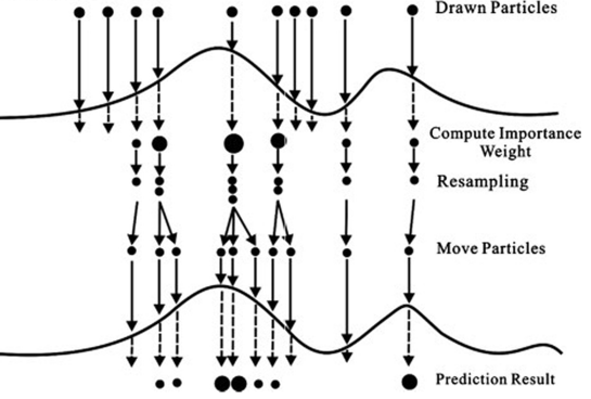
Read the picture from top to bottom: we start with particles having all the same size, which means they have equal weight $w_t^i=1/N$ . Particles are then evaluated on the density $p(y_t|x_t^i)$ depicted with a curve. The particles weight is computed and you can see that some particles have a larger size (large weight), others are smaller and some have “disappeared”, which means that their weight is negligible. At this point the particles are resampled: notice at the resampling stage the largest particle in the figure happens to be resampled three times while others fewer times. Once resampling is performed, all the resampled particles get the same size because all weights are reset to $1/N$ as described above. Now it is time to propagate the resampled particles forward to time $t+1$ : we create a new generation of particles by moving forward only the ones we have resampled. This means that some of the particles having very small weight at time $t$ will not be propagated to $t+1$ (notice in the figure, some particles do not have arrows departing from them), and the one that has been resampled three times generates three new particles. This implies that at each generation we still have $N$ particles at our disposal, even though some from the previous generation have “died”. I illustrate the use of the resampling step in the bootstrap filter.

The bootstrap filter

The bootstrap filter is the simplest example of a sequential importance sampling with resampling (SISR) algorithm. It is the “simplest” application of SISR because it assumes $h(x_{t}^i|x_{0:t-1}^i,y_{1:t}) \equiv p(x_{t}^i|x_{t-1}^i)$ , that is the law of the Markov process is used as importance sampler to propagate particles forward. This implies the already mentioned simplification for the computation of the weights, and we have

$w_t^i= \frac{1}{N} p(y_t|x_t^i;\theta) \qquad i=1,...,N.$

Notice that in the equation above we have an equality, instead of a proportionality, since after resampling we set weights to be all equal to $1/N$ , hence after resampling $w_{t-1}^i=1/N$ .

This approach is certainly very practical and appealing, but it comes at a cost. Generating particles from $p(x_{t}^i|x_{t-1}^i)$ means that these are “blind” to data, since this importance density is unconditional to $y_{1:t}$ . Hence the propagation step does not take advantage of any information carried by the data. In some scenario this produces an inefficient sampling that may result, again, in particle degeneracy. A popular alternative is the auxiliary particle filter. I do not go further into the possible improvements over the bootstrap filter however some literature is given at the end of this post.

So here is the bootstrap filter in detail.

At $t=0$ (initialize) $x^i_0\sim p(x_0)$ and assign $\tilde{w}_0^i=1/N$ , for all $i=1,...,N$ .
At the current $t$ assume to have the weighted particles $\{x_t^i,\tilde{w}_t^i\}$ .
From the current sample of particles, resample with replacement $N$ times to obtain $\{\tilde{x}_t^i,i=1,...,N\}$ .
Propagate forward $x_{t+1}^i\sim p(x_{t+1}|\tilde{x}_{t}^i)$ , for all $i=1,...,N$ .
Compute $w_{t+1}^i=p(y_{t+1}|x_{t+1}^i)$ and normalise weights $\tilde{w}_{t+1}^i={w}_{t+1}^i/\sum_{i=1}^N {w}_{t+1}^i$ .
Set $t:=t+1$ and if $t<T$ go to step 2 otherwise go to 7.
Return $\hat{p}(y_{1:T}|\theta)= \prod_{t=1}^T\biggl (\frac{1}{N}\sum_{i=1}^N w_t^i\biggr )$ .

Recall that $p(x_0)$ is the unconditional density of an arbitrary initial state $x_0$ ; this density is set by the modeller (alternatively, $x_0$ can be fixed deterministically and then all particles will propagate from a common $x_0$ ). Notice in step 5 I wrote $w_{t+1}^i=p(y_{t+1}|x_{t+1}^i)$ instead of $w_{t+1}^i=p(y_{t+1}|x_{t+1}^i)/N$ . The two formulations are completely equivalent as they only differ by a constant which is irrelevant for the purpose of assigning a weight to a particle. Also, since weights are going to be normalised, the $1/N$ is not really necessary. However if for some reason it is relevant to have a pointwise estimate of the likelihood (as opposed to e.g. optimizing it over $\theta$ ), then it is important to recover the constant, and write $\hat{p}(y_t|y_{1:t-1};\theta)=\frac{1}{N}\sum_{i=1}^N w_t^i$ . In step 7 I have explicitly reported the likelihood approximation, even though for parameter inference the product of the normalizing constants $1/N^T$ can be disregarded.

The seven steps above are the simplest version of a bootstrap filter, where the resampling is performed at every $t$ . However, the resampling adds unwanted variability to the estimate of the likelihood function. This extra variability is not really welcome as it makes the estimate more imprecise (and can affect the performance of the pseudo-marginal algorithms I will describe in future posts).

A standard way to proceed is to resample only when necessary, as given by a measure of potential degeneracy of the sequential Monte Carlo approximation, such as the effective sample size (Liu and Chen, 1998). The effective sample size takes values between 1 and $N$ and at time $t$ is approximated via $ESS = 1/\sum_{i=1}^N (\tilde{w}_t^i)^2$ . If the degeneracy at $t$ is too high, i.e. the ESS is below a specified threshold (say below $N/2$ ) then resampling is performed, otherwise no resampling is performed at time $t$ .

Finally notice that SISR (and the bootstrap filter) returns an unbiased estimate of the likelihood function. This is completely unintuitive and not trivial to prove. I will go back to this point in a future post.

Implement resampling

Coding your own version of a resampling scheme should not be necessary: popular statistical software will probably have built-in functions implementing several resampling algorithms. To my knowledge, the four most popular resampling schemes are: residual resampling, stratified resampling, systematic resampling and multinomial resampling. I mentioned above that resampling adds additional unwanted variability to the likelihood approximation. Moreover, different schemes produce different variability. Multinomial resampling is the one that gives the worse performance in terms of added variance, while residual, stratified and systematic resampling are about equivalent, though systematic resampling is often preferred because easier to implement and fast. See Douc et al. 2005 and Hol et al. 2006.

Summary

I have addressed the problem known as “particles degeneracy” affecting sequential importance sampling algorithms. I have introduced the concept of resampling, and when to perform said resampling. This produces a sequential importance sampling resampling (SISR) algorithm. Then I have introduced the simplest example of SISR, the bootstrap filter. Finally, I have briefly mentioned some results pertaining resampling schemes.

We now have a partial (though useful starting point for further self study) introduction to particle filters / sequential Monte Carlo methods for approximating the likelihood function of a state space model. We are now ready to consider Bayesian parameter inference, including practical examples.

2 Responses to Sequential Monte Carlo and the bootstrap filter

ermafl says:

April 27, 2021 at 20:01

Just wanted to say these posts were extremely helpful
– Grateful reader

LikeLike

- Jzin Ou says:
  
  December 13, 2021 at 06:32
  
  Exactly a nice blog! detail derivation, thorough discussion!
  
  LikeLike

Sequential Monte Carlo and the bootstrap filter